
The question
Indoor positioning matters most where GPS fails and the stakes are high: a warehouse robot, a firefighter in a smoke-filled corridor, a survivor under earthquake debris. Channel State Information (CSI) is the natural signal for it. Unlike RSSI, which collapses the whole channel into one number, CSI exposes amplitude and phase across every OFDM subcarrier, giving a rich fingerprint of the multipath environment.
The catch is that CSI fingerprints are not stationary in time. Collect a database on Monday, deploy on Friday, and accuracy degrades: furniture moved, humidity changed, people are standing in different places, and the receiver's automatic gain control has drifted. Formally, the test distribution is no longer the training distribution.
Can temporal covariate shift in CSI localization be neutralized at the physical layer, before the network sees the data, rather than absorbed by a larger model or patched with labelled recalibration data?
Why the prior art breaks
The dominant approach treats the CSI matrix as an image. DeepFi autoencodes CSI amplitudes; ConFi arranges CSI as time-frequency images and applies CNNs to capture local correlations across subcarriers. These work well in controlled settings, and that success is exactly the trap.
Treating the channel as a picture imports assumptions that are simply false about radio:
- Channel amplitudes are not pixels. Their magnitude carries physical units and calibration state, not perceptual intensity.
- Subcarrier indices are not spatial coordinates. Adjacency in frequency is not adjacency in space; convolutional locality encodes a neighbourhood relation that doesn't exist.
- ADC saturation is not image noise. Clipping is a deterministic, non-linear hardware signature, not a zero-mean perturbation you can augment away.
The consequence: image-based abstractions discard the multipath topology, the deterministic fingerprint of hardware non-linearity, and the temporal coherence of signal bursts, precisely the structure needed to stay robust when the environment drifts.
The second common shortcut is equally costly. Pipelines routinely discard packets from receivers whose amplifier has saturated, treating them as corrupt. On low-cost IoT hardware that can mean throwing away a large share of the data from exactly the nodes closest to the transmitter.
Hypothesis
If domain divergence is created by physics (gain drift, saturation, multipath geometry), then it can be removed by physics-aware preprocessing, restoring the i.i.d. assumption before any learning happens. Saturated packets are not noise; they are recoverable signal.
Method
The framework is a three-stage variance-reduction pipeline feeding a residual temporal network. The design principle throughout: purify the manifold first, then learn on it.
Multi-Feature Spectral Depth (MFSD) filter
Rejects non-physical artifacts, measurements that cannot correspond to a realizable propagation path, before they enter the statistics of the dataset.
Eigen-Space Consistency (ESC)
Isolates the rank-1 multipath geometry: the dominant eigen-structure of the channel that reflects room geometry rather than transient interference or receiver state.
Enhanced Correlation Alignment (CORAL)
Formally restores the i.i.d. assumption across temporally disjoint domains by aligning second-order statistics, no labels from the target day required.
1D-ResNet + Squeeze-and-Excitation + sparse Mixture-of-Experts
The purified manifolds, expanded through non-overlapping temporal augmentation, feed a residual 1D CNN with SE attention and a sparse MoE regression head predicting 2D coordinates. A softmax gate routes each sample across three experts, buying capacity that is only partially activated per sample, and therefore capacity without proportional inference cost.
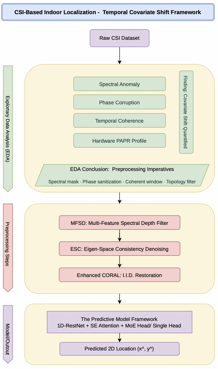
It is tempting to reach for a standard denoiser and move on. Here the preprocessing chain exists because the EDA found four specific physical failure modes, so each stage removes a named artifact rather than smoothing the signal generically. Generic denoising would have destroyed the multipath geometry the model depends on.
Inside that "predictive model" box sits the network itself, in four stages:
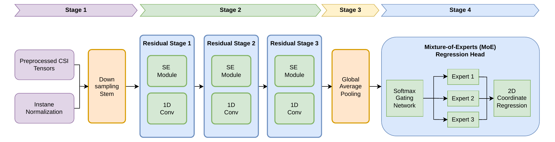
Two design choices carry most of the weight. Instance normalization defends against gain drift: normalizing per sample rather than per dataset means a receiver whose amplifier shifted overnight is rescaled before it reaches a single learned parameter.
The SE modules matter because subcarriers are not equally informative. Some sit in deep fades or carry hardware artifacts, so learned per-channel weighting beats treating all 52 as interchangeable pixels.
CORAL, interactively
Stage 3 is the conceptual core, and it is much easier to see than to read. CORAL aligns the second-order statistics of the target domain to the source: whiten the target with its own covariance, then re-colour it with the source covariance.
X′ = (X − μt) · Σt−1/2 · Σs1/2 + μs (1)
Crucially this needs no labels from the target domain, only its covariance, which can be estimated from unlabelled measurements. The demo below runs on two of my own captures from this project: the same location, same radio, same channel, recorded 19.4 minutes apart.
Temporal covariate shift, measured
ref_204_1_3500.pcap (3500 pkt) vs test_204_1_100.pcap (100 pkt) · Nexmon CSI · 52 subcarriers after removing DC, guard bands and pilots · 8-D PCA basis fitted on the reference only.
The session discriminator is the proxy 𝒜-distance: a logistic classifier trained to guess which capture a packet came from. Near 50% it cannot tell them apart: the goal. On raw features it approaches 100%: the drift is so structured that the session is trivially identifiable, which is precisely what a fingerprinting model would latch onto instead of position.
Note that mean-only alignment is not enough: first-order correction still leaves the discriminator around 60%, a clear residual signature. Only second-order alignment returns it to chance. That gap is the argument for CORAL.
The same effect appears in the paper's own diagnostics, viewed two ways: as a manifold and as a distribution:
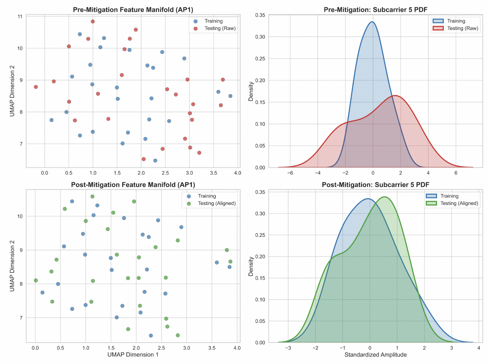
The right-hand panels are the more damning of the two. A single subcarrier's amplitude distribution has visibly different variance, not merely a different mean, which is exactly why re-centring the data is insufficient and why the alignment has to operate on second-order statistics. The post-mitigation densities overlap almost entirely.
Running that analysis offline over my own captures gives the numbers the demo reproduces live (logistic discriminator, 52-D dB-amplitude features, averaged over 15 random splits):
| Alignment | ‖Σr−Σt‖F | Session discriminator | Interpretation |
|---|---|---|---|
| None (raw features) | 767.1 | 97.6% | Sessions trivially separable |
| Mean only (first order) | 767.1 | 60.9% | Residual signature remains |
| CORAL (second order) | 3.6 | 47.6% | Indistinguishable, at chance |
The middle row is the one worth pausing on: simply re-centring the data, the obvious first fix, removes only part of the problem. The covariance structure itself carries the session identity.
Experimental design
The evaluation protocol is the part I'd defend most strongly. A random train/test split on a CSI dataset leaks temporal context and flatters every model, neighbouring packets from the same second end up on both sides of the split.
- Temporally disjoint test set. Train and test come from separate collection periods, so the model is evaluated on a genuinely unseen domain.
- Unsupervised domain generalization. No target-domain labels are used at any stage.
- Baseline. The dataset's published multi-node benchmark of 1.39 m, plus the CSILoc benchmark evaluated per node.
- Metric. Mean Distance Error (MDE) in metres for 2D coordinate regression, reported per access point rather than pooled, pooling hides which nodes fail.
Results
Two results matter more than the headline number. First, the framework beats the CSILoc benchmark on all six nodes, not on average, but individually, which is the honest way to report multi-node localization. Second, receivers that conventional pipelines discard as unusable due to ADC saturation still deliver sub-metre precision at 0.92 m: the recovery step turns thrown-away data into working infrastructure.
Why the saturated receivers were recoverable
The 0.92 m result rests on a claim that needs evidence: that packets from a clipped front end still carry position information. Establishing that took a forensic look at the raw I/Q codes, before any model was involved.
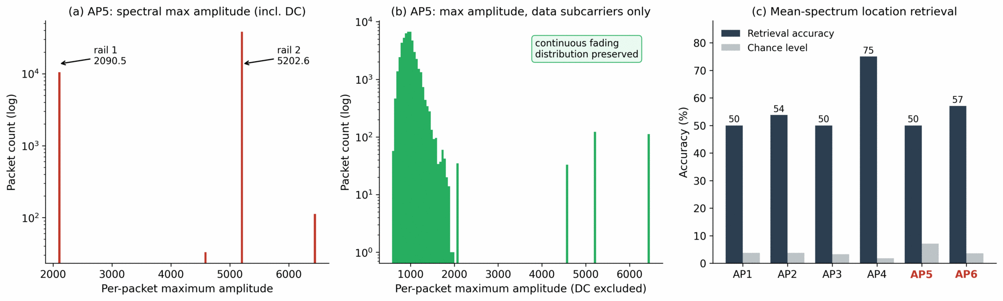
Panel (a) is the diagnosis. A random impairment would spread the spectral maximum across a continuum. Instead it snaps to two exact values, because the automatic gain control switches between discrete states and pins the LO-leakage line at DC.
On AP4–AP6 that pinned line is the spectral maximum in ≥99.7% of packets, against 58–63% on AP1 and AP3: a front end persistently driven to the top of its dynamic range.
Panel (b) is the reprieve. Remove that one artificial subcarrier and the underlying physics reappears intact. The corruption was concentrated in a component that carries no channel information at all.
| Statistic | AP1 | AP2 | AP3 | AP4 | AP5 | AP6 |
|---|---|---|---|---|---|---|
| DC is spectral max (% packets) | 58.0 | 95.9 | 63.2 | 99.8 | 99.7 | 99.7 |
| Median pinned DC amplitude | 3431 | 3661 | 3614 | 5138 | 5203 | 3924 |
| PAPR, 95th pct (excl. DC) | 4.49 | 4.55 | 4.38 | 4.89 | 3.93 | 3.98 |
| Packet–eigenpattern coherence | 0.927 | 0.938 | 0.936 | 0.933 | 0.936 | 0.935 |
| Location retrieval (%) | 50.0 | 53.8 | 50.0 | 75.0 | 50.0 | 57.1 |
| Chance level (%) | 3.8 | 3.8 | 3.3 | 1.8 | 7.1 | 3.6 |
The last two rows carry the argument. Retrieval on the saturated nodes reaches 50.0% and 57.1% against chance levels of 7.1% and 3.6%, an order of magnitude above chance, and squarely in the range of the unimpaired nodes (50.0–53.8%). Meanwhile the median packet-to-eigenpattern coherence on the saturated nodes (0.935–0.936) is statistically indistinguishable from the clean ones (0.927–0.938).
All of these statistics are computed deterministically from raw I/Q codes, before any learning. That ordering matters: it means the decision to recover saturated packets rather than discard them is justified by the physics of the capture, not retrofitted from a model that happened to work. The multipath topology survives dynamic-range compression, so the packets are recoverable information, not noise.
Headline accuracy can hide a model that has latched onto an artifact. We validated with 1D Grad-CAM over the subcarrier axis, confirming the network attends to physically meaningful regions of the channel response rather than to hardware-specific quirks, the same explainability instinct carried over from the medical-imaging work.
Latency: treating deployment as a result
An indoor positioning system that cannot run on the node is a paper, not a product. We profiled inference against the temporal window size W:
| Window (W) | Inference latency | Interpretation |
|---|---|---|
| W = 40 | 30.50 ms | Latency optimum: the operating point we recommend |
| W = 70 | +0.24 ms | Deeper temporal context for negligible additional cost |
The interesting finding is how flat that curve is: extending the window from 40 to 70 samples costs a quarter of a millisecond. Temporal context is nearly free here, which is not what you would assume from parameter count alone.
What didn't work, and what I'd caveat
These are the boundaries of the claim, stated plainly.
- Image-style abstractions were a dead end. Early experiments following the ConFi-style treatment of CSI as a 2D image plateaued: the model learned the collection session, not the geometry. This motivated the physics-aware reframing rather than deeper networks.
- CORAL only aligns second-order statistics. Where drift changes higher-order structure (a fundamentally different multipath topology after major furniture rearrangement), covariance alignment cannot recover it. It buys robustness to gain and correlation drift, not to a new room.
- Evaluated on one testbed. Results come from a single dataset's node deployment. Generalization across buildings and radio hardware families remains open.
- Saturation recovery has a floor. Recovering clipped packets restores usable precision (0.92 m) but not parity with unsaturated receivers (0.60 m). Information destroyed by clipping is not fully recoverable, only partially reconstructible from physical constraints.
What I'd do next
- Cross-building generalization. Test whether the purified manifold transfers to a testbed with different geometry and hardware, which is the real claim I would like to make.
- Online adaptation. CORAL statistics can be updated incrementally from unlabelled traffic, turning day-to-day drift correction into a continuous background process rather than a retraining event.
- Higher-order alignment. Compare against adversarial and optimal-transport domain adaptation to quantify what second-order alignment leaves on the table.
- On-device measurement. The 30.5 ms figure is a profiling result; the honest next step is measuring on the actual IoT class of hardware, with the energy budget included.
Artifacts
Related work in this line: device heterogeneity in RSSI positioning (IEEE Access, 2025), the RSSI-domain predecessor to this framework.